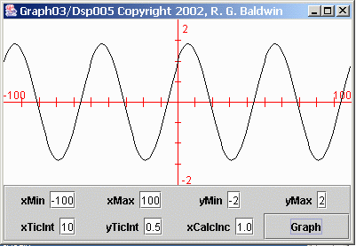
Figure 1 A sinusoidal function
Published:
December 1, 2002
By Richard G. Baldwin
DSP Programming, Notes # 100
Viewing tip
You may find it useful to open another copy of this lesson in a separate browser window. That will make it easier for you to scroll back and forth among the different figures while you are reading about them.
Supplementary material
I recommend that you also study the other lessons in my extensive collection of online programming tutorials. You will find a consolidated index of my online tutorial lessons at WWW.DickBaldwin.com.
Many physical devices (and electronic circuits as well) exhibit a characteristic commonly referred to as periodic motion.
I will use the example of a pendulum to introduce the concepts of periodic motion, harmonic motion, and sinusoids.
I will introduce you to the concept of a time series.
I will introduce you to sine and cosine functions and the Java methods that can be used to calculate their values.
I will introduce you to the concepts of period and frequency for sinusoids.
I will introduce you to the concept of radians versus cycles.
I will introduce you to the concept decomposing a time series into a (possibly very large) set of sinusoids, each having its own frequency and amplitude. We will learn much more about this in a subsequent lesson when we discuss frequency spectrum analysis.
I will introduce you to the concept of composition, where any time series can be created by adding together the correct (possibly very large) set of sinusoids, each having its own frequency and amplitude.
I will show you examples of using composition to create a square waveform and a triangular waveform.
I will identify some real-world examples of frequency filtering and real-time spectral analysis
The most difficult decision that I must make for this series is to decide where to begin. I need to begin at a sufficiently elementary level that you will understand everything that you read. So, before getting into the actual topic of digital signal processing, I'm going to take you back to some elementary physics and mathematics concepts and discuss periodic motion.
Many physical devices (and electronic circuits as well) exhibit a characteristic commonly referred to as periodic motion. This includes pendulums, acoustic speakers, springs, vocal cords, etc.
Motion of a pendulum
For example, consider the pendulum on a grandfather clock. Once you start the pendulum swinging, it will swing for a long time (actually, the spring in the clock gives it a little kick during each repetition, so it will continue to swing until the spring runs down).
The most important characteristic of the motion of the pendulum is that every repetition takes almost exactly the same amount of time. In other words, the period of time during which the pendulum swings from one side to the other is very constant. That is the source of the term periodic motion.
A bag of sand
Even without the spring to help it along, a pendulum swinging in a low-friction environment will swing for a long time. Visualize a pendulum consisting of a bag of sand tied to the end of a long rope suspended from your ceiling (sheltered from the wind). Assume that the bag is filled with colored sand, and that it has a small hole in the bottom. Assume that you start it swinging in a back-and-forth motion (no circular motion).
The sand traces out a pattern
As the bag of sand swings back and forth, a little bit of sand will leak out of the hole and land on the floor below. The sand will trace out a line, which is parallel to the direction of motion of the bag of sand.
Now assume that you carefully drag a carpet across the floor under the bag at a uniform rate, perpendicular to the direction of motion of the bag. This will cause the sand that leaks from the bag to trace out a zigzag pattern on the carpet very similar to the curved line shown in Figure 1.

Figure 1 A sinusoidal function
A sinusoidal function
The shape of the curve shown in Figure 1 is often referred to as a sinusoidal function.
In this assumed scenario, the bag is swinging back and forth along the
vertical axis in Figure 1, and the carpet is being dragged along the horizontal
axis. The motion of the bag causes the sand to be leaked in a
back-and-forth zigzag pattern. The motion of the carpet causes that
pattern to be elongated along the horizontal axis.
|
Figure 1 is a plot of the following Java expression: Math.cos(2*pi*x/50) + Math.sin(2*pi*x/50) Math in the above expression is the name of a Java library that provides methods for computing sine, cosine, and various other mathematical functions. The asterisk (*) in the above expression means multiplication. The reference to pi in the above expression is a reference to the mathematical constant with the same name. The image in Figure 1 was produced using a Java program named Graph03, which I will describe in a future tutorial lesson. |
Harmonic motion
The kind of motion exhibited by a simple pendulum is often referred to as periodic motion in general, and simple harmonic motion in particular.
Other devices that exhibit periodic motion may exhibit more complex harmonic
motion. For example, Figure 2 illustrates a more complex form of harmonic
motion.
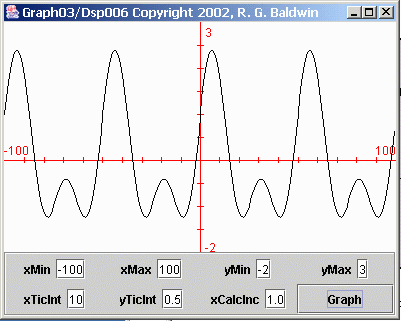
Figure 2 Complex harmonic motion
As you can see, the positive excursions are greater than the negative
excursions in Figure 2. In addition, the negative excursions exhibit some
ripple that is not exhibited by the positive excursions.
|
Figure 2 is a plot of the following Java expression: Math.cos(2*pi*x/50) + Math.sin(2*pi*x/50) + Math.sin(2*pi*x/25); |
Sinusoids
Figure 1 shows a curve whose shape is commonly referred to as a sinusoid. Eliminating the syntax required by the Java programming language, the expression used to produce the data plotted in Figure 1 was:
f(x) = cos(2*pi*x/50) + sin(2*pi*x/50)
As you can see, this function is composed of two components, one cosine component and one sine component.
Separate the cosine and sine components
Figure 3 shows separate plots of the two components that were added together to produce the plot in Figure 1.
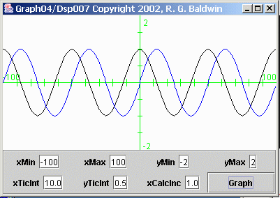
Figure 3 Separate cosine and sine functions
Plotting separate sine and cosine functions
The black curve in Figure 3 shows the cosine function produced by evaluating and plotting the following equation:
f(x) = cos(2*pi*x/50)
The blue curve shows the sine function produced by evaluating and plotting the following equation:
g(x) = sin(2*pi*x/50)
The point-by-point sum of these two curves would produce the sinusoidal curve shown in Figure 1.
Time varying functions
Many processes produce functions whose values vary over time. For example, the temperature in your office is a function that varies continuously with time.
(The temperature in your office is probably not a periodic function because the temperature probably doesn't repeat its values on any periodic basis).
Sampled data
If you were to measure and record the temperature in your office once each minute, you could plot the recorded values in the manner shown in Figures 1 through 3. You could plot the temperature along the vertical axis against time (or sample number) along the horizontal axis.
A common name for sampled data of this type is time series. That name reflects the fact that your data is a recording of the temperature values for a series of measurements that occur over time. (I will have quite a lot more to say about time series in future lessons.)
The period of the sine and cosine functions
Figure 4 is very similar to Figure 3. However, there is one major difference. In Figure 3, the repetition period of the sine and cosine functions is the same. In other words, the shape of the sine function is the same as the shape of the cosine function. They are simply shifted relative to one another along the horizontal axis.
Each of the curves in Figure 3 has the same period, where the period is the horizontal distance from one peak to the next.
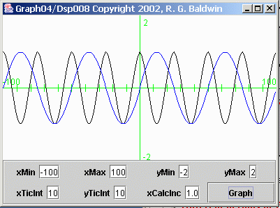
Figure 4 Sinusoid with frequency modification
Different periods or frequencies
The black curve in Figure 4 was produced by evaluating and plotting the following equation:
f(x) = cos(2*pi*x/25)
The blue curve in Figure 4 was produced by evaluating and plotting the following equation:
g(x) = sin(2*pi*x/50
Note that the periods (frequencies) for the black cosine curve and the blue sine curve in Figure 4 are not the same. The period for the black curve is one-half that of the blue curve. Stated differently, the frequency of the black curve is twice that of the blue curve.
(Frequency and period are reciprocals of one another. Period is a measure of the time required to complete one cycle of the function. Frequency is a measure of the number of cycles that are completed in a given amount of time, usually one second.)
Modified arguments
This difference exists because I modified the argument in the equation for the cosine function relative to the sine function. In particular, I halved the value in the denominator in the cosine argument relative to the denominator in the sine argument.
This caused the period of the cosine function to be only half as long as the period for the sine function. Stated differently, this caused the frequency of the cosine function to be twice the frequency of the sine function.
Why does pi appear in the arguments?
Although it isn't obvious, for any given value of x, the arguments for the sine and cosine functions shown above are angular measurements in radians.
Most programming languages provide methods for computing the sine and the cosine values for an angle given in radians. That is true for Java, and it is also true for the plotting software used to produce these graphs. (These graphs were produced using a Java program.)
Radians versus cycles
One cycle constitutes 360 degrees.
(For example, this is the number of degrees that the big hand on a clock must traverse to begin at the 12 and make one complete cycle around the clock face and back to the 12.)
Beyond one cycle, the values of the sine and cosine functions repeat.
An angle of one radian is approximately equal to 57.3 degrees, and is exactly equal to 360 degrees divided by 2*pi. Therefore, in order to use a method that expects to receive an angle in radians, it is necessary to apply the correction factor of 2*pi as shown above to convert from cycles to radians.
The horizontal scale
The horizontal scale in Figure 4 extends from minus 100 units to plus 100 units with a value of 0 in the center.
A tic mark appears every ten units. For x equal to 25, the argument for the cosine function equals 2*pi radians, or 360 degrees. A close examination of Figure 4 shows that the cosine curve goes through one full cycle between an x value of 0 and an x value of 25. Beyond that, the cosine function simply repeats.
Similarly, for x equal to 50, the argument for the sine function equals 2*pi radians, or 360 degrees. Again, a close examination of Figure 4 shows that the sine curve goes through one full cycle between an x value of 0 and an x value of 50. Beyond that, the sine function simply repeats.
The argument to the sine and cosine functions
If you think of x as being a measurement of time in seconds, and 1/n being a measurement of frequency in cycles/second, the arguments to the sine and cosine functions can be viewed as:
2*pi(radians/cycle)*(x sec)*(1/n)( cycle/sec)
If you cancel out like terms, this reduces to:
2*pi(radians)*(x )*(1/n )
Thus, with a fixed value of n, for each value of x, the argument represents an angle in radians, which is what is required for use with the functions of the Java Math library.
Where does sin(arg) equal zero?
The value of the sine of an angle goes through zero at every integer multiple of pi radians. This explanation will probably make more sense if you refer back to Figure 3.
The curve in Figure 3 was calculated and plotted for n equal to 50. The sine curve has a zero crossing for every value of x such that x is a multiple of n/2, or 25.
Where are the peaks in the cosine function?
Similarly, the peaks in the cosine curve in Figure 3 occur for every value of x such that x is a multiple of n/2, or 25.
Composition and decomposition
In theory, it is possible to decompose any time series into a number (quite possibly a very large number) of sine and cosine functions each having its own amplitude and frequency. (In a future lesson, we will learn how this is possible using a Fourier series or a Fourier transform.)
Conversely, it is theoretically possible to create any time series by adding together just the right combination of sine and cosine functions, each having its own amplitude and frequency.
An approximate square waveform
As an example of composition, suppose that I need to create a time series that approximates a square waveform, as shown at the bottom of Figure 6.
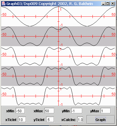
Figure 5 An approximate square waveform
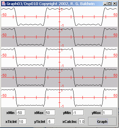
Figure 6 An improved approximate square waveform
I can create such a waveform by adding together the correct combination of sinusoids, each having its own frequency and amplitude.
Successive approximations
The ten curves plotted in Figures 5 and 6 show successive approximations to the creation of the desired square waveform. The bottom curve in Figure 6 is a plot of the following sinusoidal expression containing the algebraic sum of ten sinusoidal terms.
cos(2*pi*x/50)
- cos(2*pi*x*3/50)/3
+ cos(2*pi*x*5/50)/5
- cos(2*pi*x*7/50)/7
+ cos(2*pi*x*9/50)/9
- cos(2*pi*x*11/50)/11
+ cos(2*pi*x*13/50)/13
- cos(2*pi*x*15/50)/15
+ cos(2*pi*x*17/50)/17
- cos(2*pi*x*19/50)/19
Each curve contains more sinusoidal terms
The top curve in Figure 5 is a plot of only the first sinusoidal term shown above. It is a pure cosine curve.
Each successive plot, moving down the page in Figures 5 and 6, adds another term to the expression being plotted, until all ten terms are included in the bottom curve in Figure 6.
Reasonably good approximation
As you can see, the bottom curve in Figure 6 is a reasonably good approximation to a square wave, but it is not perfect.
(A perfect square wave would have square corners, a flat top, no ripple, and perfectly vertical sides.)
Each term improves the approximation
If you start at the top of Figure 5 and examine the successive curves, you will see that the approximation to a square wave improves as each new sinusoidal term is added.
In theory, it would be possible to produce a perfect square wave in this fashion. Unfortunately, an infinite number of sinusoidal terms would be required to achieve the square corners, flat top, no ripples, and vertical sides of the perfect square wave. In practice, we normally have to make do with something less than perfect.
The first five sinusoidal terms
Figure 7 shows individual plots of the first five sinusoidal terms required to approximate the square wave.
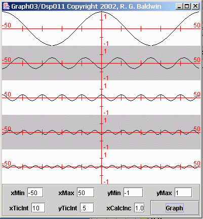
Figure 7 First five sinusoidal components of a square waveform
Each of the terms in the previous expression has an associated algebraic sign.
(You may have noticed that the sign applied to every other term in the expression is negative, causing every other term to plot upside down in Figure 7.)
The bottom curve in Figure 5 is the point-by-point sum of the five curves shown in Figure 7.
A side-by-side comparison
If you view Figure 7 side-by-side with Figure 5, you should be able to see how the sinusoidal terms add and subtract to produce the desired result. For example, the subtraction of the second sinusoidal term from the first sinusoidal term knocks the peaks off the first term and produces a noticeable shift from a cosine towards a square wave.
An approximate triangular waveform
As another example of composition, suppose that I need to create a time series that approximates a triangular waveform, as shown at the bottom of Figure 8.
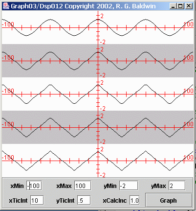
Figure 8 A triangular waveform
I can create such a waveform by adding together the right combination of sinusoids, each having its own amplitude and frequency.
Five sinusoids
The time series at the bottom of Figure 8 was created by adding together five cosine waves, each having the amplitude and frequency values shown in the following equation:
f(x) = cos(2*pi*x/50)
+ cos(2*pi*x*3/50)/9
+ cos(2*pi*x*5/50)/25
+ cos(2*pi*x*7/50)/49
+ cos(2*pi*x*9/50)/81
Intermediate waveforms
The top waveform in Figure 8 is a plot of the cosine curve created from the sinusoidal first term in the expression shown above.
The second waveform from the top in Figure 8 is the sum of the first two terms in the above expression.
The third waveform is the sum of the first three terms. By this point, the plot has begun to resemble a triangular waveform in a significant way.
The fourth waveform is the sum of the first four terms, and the fifth waveform is the sum of all five terms.
By examining the waveforms from top to bottom in Figure 8, you can see how the addition of each successive term causes the resulting waveform to more closely approximate the desired triangular shape.
Good result with only five terms
Figure 8 shows that only five terms are required to produce a fairly good approximation to a triangular waveform.
A comparison of Figure 8 with Figure 5 shows that five terms are much more effective in approximating a triangular waveform than were the five terms in approximating a square waveform. The triangular waveform is easier to approximate because it doesn't have a flat top and vertical sides.
Other waveforms exhibit greater or lesser degrees of difficulty in creation through composition.
The individual terms
I'm not going to attempt to plot the individual sinusoidal terms in the triangular waveform. After the first couple of terms, they have such a small amplitude that it is difficult to see them.
So what, you say?
By now, you are may be saying "So what?" What in the world does DSP have to do with bags of sand with holes in the bottom? The answer is everything.
Almost everything that we will discuss in the area of DSP is based on the premise that every time series, whether generated by sand leaking from a bag onto a moving carpet, or acoustic waves generated by your favorite rock band, can be decomposed into a large (possibly infinite) number of sine and cosine waves, each having its own amplitude and frequency.
A practical example
You have probably seen, the kind of stereo music component commonly known as an equalizer. An equalizer typically has about a dozen adjacent slider switches that can be moved up and down to cause the music that you hear to be more pleasing. This is a crude form of frequency filter.
Many equalizers also have a set of vertical display lights that dance up and down as your music is playing. This is a crude form of a frequency spectrum analyzer.
The frequency filters
The purpose of each slider is to attenuate or amplify a band of adjacent frequencies (sine and cosine components, each having its own amplitude and frequency), before they make their way to the output amplifier and impinge on the system speakers. Thus, while you don't have the ability to attenuate or amplify each individual sine and cosine component, you do have the ability to attenuate or amplify them in groups.
In subsequent lessons, we will learn how to use digital filters to attenuate or amplify the sine and cosine waves that make up a time series.
The spectrum analyzer
At an instant in time, the height of one of the vertical display lights is an indication of the combined power of the sine and cosine waves contained in a small band of adjacent frequencies.
In subsequent lessons, you will learn how to use Fourier analysis to perform spectral analysis on time series.
I used the example of a pendulum to introduce the concepts of periodic motion, harmonic motion, and sinusoids.
I introduced you to the concept of a time series.
I introduced you to sine and cosine functions and the Java methods that can be used to calculate their values.
I told you that almost everything we will discuss in this series on DSP is based on the premise that every time series can be decomposed into a large number of sinusoids, each having its own amplitude and frequency.
I introduced you to the concepts of period and frequency for sinusoids.
I introduced you to the concept of radians versus cycles.
I introduced you to the concept decomposing a time series into a (possibly very large) set of sinusoids, each having its own frequency and amplitude. I told you that we will learn more about this later when we discuss frequency spectrum analysis.
I introduced you to the concept of composition, where any time series can be created by adding together the correct (possibly very large) set of sinusoids, each having its own frequency and amplitude.
I showed you examples of using composition to create a square waveform and a triangular waveform.
I identified the frequency equalizer in your audio system as an example of frequency filtering.
I identified the frequency display that may appear on your frequency equalizer as an example of real-time spectrum analysis
Copyright 2002, Richard G. Baldwin. Reproduction in whole or in part in any form or medium without express written permission from Richard Baldwin is prohibited.
Richard has participated in numerous consulting projects and he frequently provides onsite training at the high-tech companies located in and around Austin, Texas. He is the author of Baldwin's Programming Tutorials, which has gained a worldwide following among experienced and aspiring programmers. He has also published articles in JavaPro magazine.
In addition to his programming expertise, Richard has many years of practical experience in Digital Signal Processing (DSP). His first job after he earned his Bachelor's degree was doing DSP in the Seismic Research Department of Texas Instruments. (TI is still a world leader in DSP.) In the following years, he applied his programming and DSP expertise to other interesting areas including sonar and underwater acoustics.
Richard holds an MSEE degree from Southern Methodist University and has many years of experience in the application of computer technology to real-world problems.
-end-